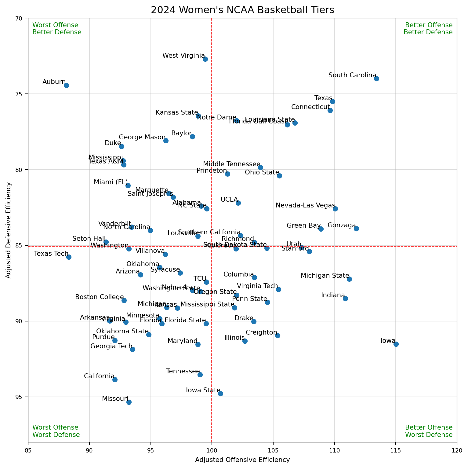
Statistical Analysis of 2024 Women’s College Basketball

sports

data

Published

May 22, 2023

Code

# Create dataframe for offensive and defensive team stats
team_stats = pd.merge(raw_stats, raw_opponent_stats, on="School", how="inner")
team_stats.columns = team_stats.columns.str.replace('_x', '')

team_stats = team_stats[['School', 'Overall_SRS', 'Overall_SOS', 'Overall_W', 'Overall_L',
                         'Team_FG', 'Team_FGA', 'Team_3P', 'Team_3PA',  'Team_FTA', 'Team_ORB', 'Team_TRB', 'Team_TOV',
                         'Opponent_FG', 'Opponent_FGA', 'Opponent_3P', 'Opponent_3PA',  'Opponent_FTA', 'Opponent_ORB', 'Opponent_TRB', 'Opponent_TOV']].copy()

# Set datatype
team_stats = team_stats.astype({
    'Overall_SRS': 'float',
    'Overall_SOS': 'float',
    'Overall_W': 'int',
    'Overall_L': 'int'
})

# Cast all other columns to float
cast_to_float = team_stats.columns[5:]
team_stats[cast_to_float] = team_stats[cast_to_float].astype(float)

team_stats.dtypes

# Divide teams into SRS percentile
bins = [0, 0.25, 0.5, 0.8, 1]
labels = ['Bottom 25%', '25th-50th %', '50th-80th %', 'Top 20%']

team_stats['Pct_Group'] = pd.qcut(team_stats['Overall_SRS'], q=bins, labels=labels)

Statistical Analysis of 2024 Women’s College Basketball

Unlike Men’s College Basketball, statistical analysis on the Women’s game is relatively sparse. Since analysis for the Men’s game is widely available and well documented, I’ve applied some of the most popular methodologies to basic team stats for the Women’s game to better understand how strongly corralated the four factors are with the teams simple rating system, measure the offsive and defensive efficiency of each team, and visualize the strengths (and weaknesses) of each team. Let’s dive in!

Four Factors of Basketball

The Four Factors designed by Dean Oliver in “Basketball on Paper” is considered the moneyball of Basketball to measure a team’s success. While these stats can be found calculated in Sports Reference’s Advanced School Stats, we’ll calculated them to see how they correlate with the teams simple rating system then use the four factors to measure the offensive and defensive efficiency of each team.

These four factors are:

Shooting the ball well measured by effective Field Goal % (eFG%)

Code

# Calculate both offensive and defensive effective field goal percentage
team_stats['Calc_Off_eFG%'] = (team_stats['Team_FG'] + 0.5 * team_stats['Team_3P']) / team_stats['Team_FGA']
team_stats['Calc_Def_eFG%'] = (team_stats['Opponent_FG'] + 0.5 * team_stats['Opponent_3P']) / team_stats['Opponent_FGA']

The effective field goal % captures the teams ability to shoot the ball. Because at the end of the game, the team with the most points wins. This is calculated as Field Goals Made + 0.5 * 3-pointers Made) / Field Goals Attempted. Unlike FG%, this calculation adds 50% more credit for 3-pointers made, since they are worth more points.

** Avoiding turnovers - Turnover % **

Code

# Calculate Pace or Possessions
team_stats['Pace'] = team_stats['Team_FGA'] - team_stats['Team_ORB'] + team_stats['Team_TOV'] + (0.475 * team_stats['Team_FTA'] )

# Calculate Turnover %
team_stats['Calc_Off_TOV%'] = team_stats['Team_TOV'] / team_stats['Pace']
team_stats['Calc_Def_TOV%'] = team_stats['Opponent_TOV'] / team_stats['Pace']

Giving the ball away too often is a surefire way to lose a game. What percentage of possessions end in a turnover?

Turnover % = Turnovers / Possessions

Second changes to score: Offensive rebound %

Code

# Create the defensive rebound column
team_stats['Team_DRB'] = team_stats['Team_TRB'] - team_stats['Team_ORB']
team_stats['Opponent_DRB'] = team_stats['Opponent_TRB'] - team_stats['Opponent_ORB']

# Calculate offensive rebound %
team_stats['Calc_ORB%'] = team_stats['Team_ORB'] / (team_stats['Team_ORB'] + team_stats['Opponent_DRB'])
team_stats['Calc_Opp_ORB%'] = team_stats['Opponent_ORB'] / (team_stats['Opponent_ORB'] + team_stats['Team_DRB'])

Offensive rebounds are a second change at scoring. So of the total rebounds happening while a team is on offense, how many are the offensive team getting them.

Offensive Rebounding % = Offensive Rebounds / (Offensive Rebounds + Opponent’s Defensive Rebounds)

Getting to the foul line: Free throw rate

Code

team_stats['Calc_Off_FTR'] = team_stats['Team_FTA'] / team_stats['Team_FGA']
team_stats['Calc_Def_FTR'] = team_stats['Opponent_FTA'] / team_stats['Opponent_FGA']

Free throws are yet another attempt to score. So getting fouled
Free Throw Rate = Free Throws Attempts / Field Goal Attempts

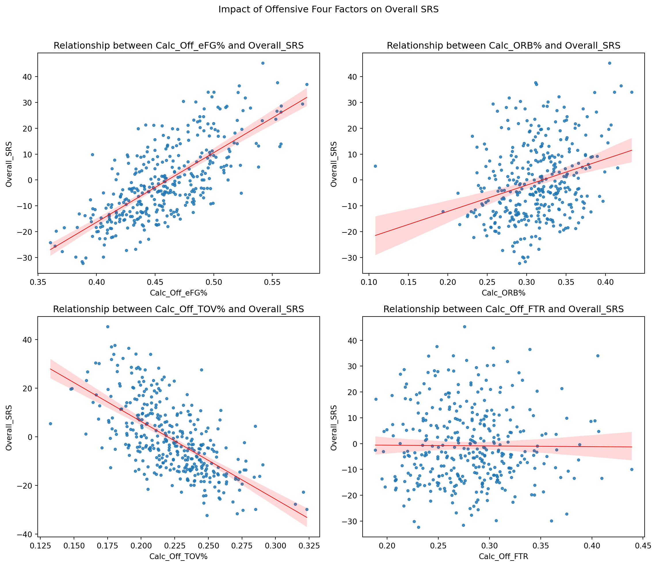
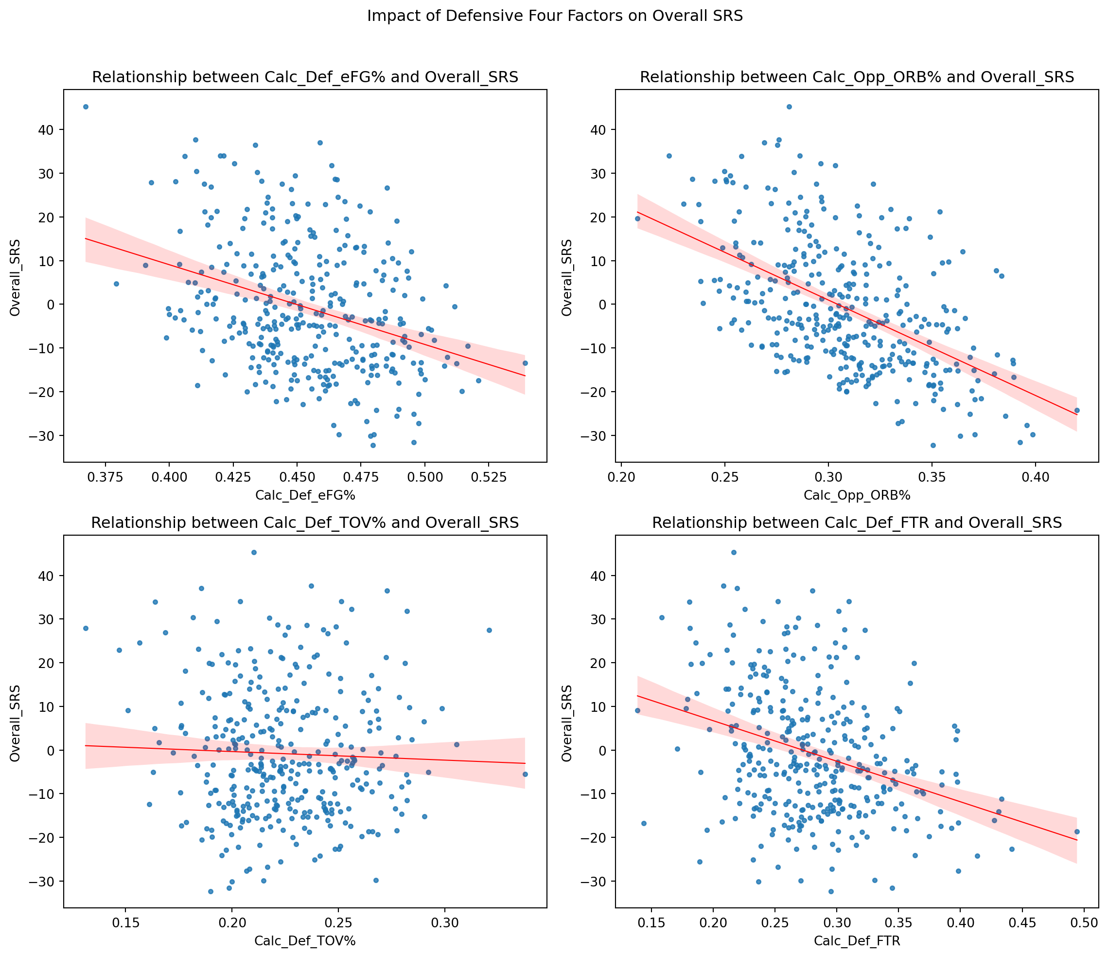
Relationship of Four Factors with Overall SRS

Once each of these metrics has been calculated, let’s evaulate the impact each metric has on the overall simple rating system of the team.

Code

# Set up the figure with four subplots
fig, axes = plt.subplots(2, 2, figsize=(12, 10))  # 2x2 grid

off_four_factors = team_stats[['School', 'Overall_SRS', 'Calc_Off_eFG%', 'Calc_ORB%', 'Calc_Off_TOV%', 'Calc_Off_FTR']]

# List of offensive factors
offensive_factors = ['Calc_Off_eFG%', 'Calc_ORB%', 'Calc_Off_TOV%', 'Calc_Off_FTR']

# Loop through the factors and plot each one against 'Overall_SRS'
for ax, factor in zip(axes.flatten(), offensive_factors):
    sns.regplot(
        data=off_four_factors,
        x=factor,
        y='Overall_SRS',
        ax=ax,
        scatter_kws={'s': 10},
        line_kws={'color': 'red', 'linewidth': 0.8}
    )
    ax.set_title(f'Relationship between {factor} and Overall_SRS')

plt.suptitle('Impact of Offensive Four Factors on Overall SRS', y=1.02)
plt.tight_layout()
plt.show()

Code

# Set up the figure with four subplots
fig, axes = plt.subplots(2, 2, figsize=(12, 10))  # 2x2 grid

def_four_factors = team_stats[['School', 'Overall_SRS', 'Calc_Def_eFG%', 'Calc_Opp_ORB%', 'Calc_Def_TOV%', 'Calc_Def_FTR']]

# List of defensive factors
defensive_factors = ['Calc_Def_eFG%', 'Calc_Opp_ORB%', 'Calc_Def_TOV%', 'Calc_Def_FTR']

# Loop through the factors and plot each one against 'Overall_SRS'
for ax, factor in zip(axes.flatten(), defensive_factors):
    sns.regplot(
        data=def_four_factors,
        x=factor,
        y='Overall_SRS',
        ax=ax,
        scatter_kws={'s': 10},
        line_kws={'color': 'red', 'linewidth': 0.8}
    )
    ax.set_title(f'Relationship between {factor} and Overall_SRS')

plt.suptitle('Impact of Defensive Four Factors on Overall SRS', y=1.02)
plt.tight_layout()
plt.show()

In all calculations, I use per game average since as a basketball fan, it allows me to reason about the data and catch mistakes easier. For example, if free throw attemps is 78, I’m able to recognize and issue witih my data. To increase accuracy calculations could be done on a per game basis before averaged out.

Sources: https://kenpom.com/blog/four-factors/

Offensive & Defensive Efficiency

In order for us to measure the offensive and defensive efficiency of each team, we’ll first calculate these stats for each team, this is their offense. For defense, we’ll calculate how well their opponents do in each of these stats when playing against them.

team_stats['Calc_Off_Eff'] = 32.333 + 1.55 * team_stats['Calc_Off_eFG%'] * 100 \
                                    + 0.47 * team_stats['Calc_ORB%'] * 100 \
                                    - 1.55 * team_stats['Calc_Off_TOV%'] * 100 \
                                    + 0.19 * team_stats['Calc_Off_FTR'] * 100

sorted_df = team_stats.sort_values(by='Calc_Off_Eff', ascending=False)
sorted_df[['School', 'Overall_SRS', 'Calc_Off_Eff', 'Calc_Off_eFG%', 'Calc_ORB%', 'Calc_Off_TOV%', 'Calc_Off_FTR']].head(10)

	School	Overall_SRS	Calc_Off_Eff	Calc_Off_eFG%	Calc_ORB%	Calc_Off_TOV%	Calc_Off_FTR
124	Iowa NCAA	37.05	115.024700	0.579465	0.312408	0.177928	0.303698
270	South Carolina NCAA	45.27	113.435192	0.541765	0.405128	0.175164	0.275686
102	Gonzaga NCAA	26.30	111.769560	0.557175	0.388557	0.192770	0.246925
174	Michigan State NCAA	26.69	111.204764	0.553755	0.262712	0.160003	0.289095
121	Indiana NCAA	29.50	110.880181	0.575790	0.257436	0.182287	0.287092
194	Nevada-Las Vegas NCAA	19.63	110.066279	0.523977	0.318841	0.147565	0.231782
302	Texas NCAA	36.47	109.837609	0.521739	0.419800	0.190606	0.339384
59	Connecticut NCAA	37.65	109.648191	0.554330	0.311306	0.180385	0.248543
105	Green Bay NCAA	14.22	108.897663	0.536096	0.296651	0.164052	0.260803
289	Stanford NCAA	33.90	107.932516	0.520687	0.386273	0.179534	0.240317

team_stats['Calc_Def_Eff'] = 32.333 + 1.55 * team_stats['Calc_Def_eFG%'] * 100 \
                                    + 0.47 * team_stats['Calc_Opp_ORB%'] * 100 \
                                    - 1.55 * team_stats['Calc_Def_TOV%']* 100 \
                                    + 0.19 * team_stats['Calc_Def_FTR'] * 100

sorted_df = team_stats.sort_values(by='Calc_Def_Eff', ascending=True)
sorted_df[['School', 'Overall_SRS', 'Calc_Def_Eff', 'Calc_Def_eFG%', 'Calc_Opp_ORB%', 'Calc_Def_TOV%', 'Calc_Def_FTR']].head(10)

	School	Overall_SRS	Calc_Def_Eff	Calc_Def_eFG%	Calc_Opp_ORB%	Calc_Def_TOV%	Calc_Def_FTR
202	Norfolk State NCAA	1.29	69.918558	0.417879	0.296595	0.305444	0.327273
345	West Virginia NCAA	27.52	72.701254	0.444087	0.321665	0.320728	0.322600
83	Fairfield NCAA	5.03	73.152050	0.407407	0.280582	0.268881	0.324217
270	South Carolina NCAA	45.27	73.995298	0.367242	0.280952	0.210197	0.216605
16	Auburn NCAA	19.91	74.435290	0.416424	0.303191	0.281138	0.362260
293	Stony Brook	8.96	74.558590	0.390671	0.278618	0.228701	0.211856
305	Texas A&M-Corpus Christi NCAA	-2.34	74.704027	0.400053	0.303388	0.251206	0.265284
114	Howard	-7.69	75.147372	0.398896	0.321820	0.262852	0.347472
205	North Carolina A&T	-0.95	75.214453	0.399694	0.300813	0.248231	0.277182
302	Texas NCAA	36.47	75.503534	0.433592	0.275223	0.272871	0.280175

Code

top_20 = team_stats[team_stats['Pct_Group'] == "Top 20%"]
top20_4f = top_20[['School', 'Overall_SRS', 'Pace',
                   'Calc_Off_Eff', 'Calc_Off_eFG%', 'Calc_ORB%', 'Calc_Off_TOV%', 'Calc_Off_FTR',
                   'Calc_Def_Eff', 'Calc_Def_eFG%', 'Calc_Opp_ORB%', 'Calc_Def_TOV%', 'Calc_Def_FTR']].copy()


fig, ax = plt.subplots(figsize=(12,12))

# Assign values
labels = top20_4f.School
x = top20_4f.Calc_Off_Eff
y = top20_4f.Calc_Def_Eff

# Set mean
ax.axvline(x=x.mean(), linestyle='--', color='red')
ax.axhline(y=y.mean(), linestyle='--', color='red')

# Plot data
for x0, y0, label in zip(x, y, labels):
  plt.text(x0, y0, label, fontsize=8, ha='right', va='bottom')

plt.scatter(x, y)

# Add grid
ax.grid(zorder=0, alpha=0.4)
ax.set_axisbelow(True)

ax.set_xlim(85, 120)
ax.set_ylim(98, 70)

# Add labels and text
ax.set_xlabel('Adjusted Offensive Efficiency')
ax.set_ylabel('Adjusted Defensive Efficiency')

ax.text(0.99, 0.01, 'Better Offense\nWorst Defense',
        verticalalignment='bottom', horizontalalignment='right',
        transform=ax.transAxes,
        color='green', fontsize=12)

ax.text(0.99, 0.99, 'Better Offense\nBetter Defense',
        verticalalignment='top', horizontalalignment='right',
        transform=ax.transAxes,
        color='green', fontsize=12)

ax.text(0.01, 0.99, 'Worst Offense\nBetter Defense',
        verticalalignment='top', horizontalalignment='left',
        transform=ax.transAxes,
        color='green', fontsize=12)

ax.text(0.01, 0.01, 'Worst Offense\nWorst Defense',
        verticalalignment='bottom', horizontalalignment='left',
        transform=ax.transAxes,
        color='green', fontsize=12)

ax.set_title('2024 Women\'s NCAA Basketball Tiers')

Text(0.5, 1.0, "2024 Women's NCAA Basketball Tiers")

etsaii

Relationship of Four Factors

Once we have all four factors calculated, both for offense and defense, we can see how each factor impacts their SRS rating.

In many of the analysis, we’ll also compare Sports Reference’s Simple Rating System (SRS) with the stats that we calculate. The Overall SRS, “takes into account average point differential and strength of schedule”, where zero is average and a high positive number signals a strong team.

Data Sources: Sports Reference: https://www.sports-reference.com/cbb/seasons/women/2024-ratings.html Massey Rating: https://masseyratings.com/cbw/ncaa-d1/ratings Sokol’s LRMC ratings: https://www2.isye.gatech.edu/~jsokol/lrmcW/ Moore’s ratings: https://sonnymoorepowerratings.com/w-basket.htm